|
An Engineer’s Approach to Design of Experiments
|
By Dr. Nicolo Belavendram
Design and Production, Faculty of Engineering, University of Malaya
|
Abstract
|
|
Design of Experiments per se has been a major contribution to science and technology since the time Fisher introduced the concept in the 1940s. Deming literally cursed variation as the cause of customer dissatisfaction and advocated the Deming Philosophy to reduce variation. Taguchi formulated an elegant relationship between the specification and the quality loss (with some degree of criticism). One important aspect of Design of Experiments has been the problem of making Design of Experiments a tool that is simple enough for the average engineer in a production facility to use it without tears and not forgetting to produce a reasonable report of what was done. Without proper documentation of the experimental process, the learning curve in product and process optimization goes back before the advent of papyrus. With modern Information Communications Technology, conducting good experiments should no longer be limited to the select few with their Masters or even Doctorate degrees. The focus of Design of Experiments as Fisher would have advocated would be solve problems rather than dwelling in the infinite (or infinitesimal) beauty of statistical residual estimation. In this paper, the author describes an engineering (and humane) approach to Design of Experiments.
|
|
Keywords: design of experiments, quality characteristics, quality loss function, parameter diagram, experimental design, response table, response graph, analysis of variance, optimum factor selection, confirmation experiment, predicted value, Minitab, ICT-M, Mendenhall, Montgomery, Taguchi.
|
|
Legend has it that the citizens of Delos (circa 430 BC) consulted the oracle of Apollo to end a plague. To this the oracle responded that the citizens must build an altar that was twice the size. The citizens religiously built an altar that had twice the length, twice the width and twice the height. Alas, this resulted in 8 X increase and a corresponding increase in the plague and the citizens later found (i.e. by trial and error) that the oracle meant the volume to be doubled. The scribes (shall we say engineers of the day) now had a problem: how does one double a cube?
|
|
Unfortunately, the scribes had no immediate solution to the problem. Indeed they did not have the right tool to solve the problem. But the citizens demanded the problem solved. The scribes on the other claimed a solution did not exist. Even today, if a perfect double of the cube is required, it is practically impossible because the cube root of two is not a rational number.
|
|
How are we different 2500 years later? The problem is one of evaluating a response to fifteen decimal places when in fact the industrial response is operating at 60% efficiency and fluctuates 10 percentage points by the day. No one is advocating a wrong model of use. Basic mathematical and statistical assumptions must be met. However, instead of levelling a whole lot of “statistical perfectionism” perhaps a small portion of this resource could be used to make the method "engineering friendly".
|
|
Today, there are numerous tools to help engineers solve design issues. More specifically, software tools for Design of Experiment abound including notable software such as Minitab, SigmaStat, ExcelStat, etc. While powerful in their own right, most of this software is trained on statistical rigour. For example, the user may be asked to provide generators, number of center points or blocks, etc. or asked for information on the principal fraction or resolution. There are also options. Would you like to fold on all factors or just one? How would you like the results, with the alias table and defining relation?
|
|
No wonders books on "Statistics for Fools" and "Computers for Idiots" are so popular. How is the average engineer expected to meet his office obligations and conduct industrial experimentation at the same time? How would a company provide such training for its workforce. Should a company put so much of its resources on basic education?
|
|
It is here that one can safely say that Taguchi made a great impact in the way industrial engineers related experimental design which had never before been advocated. Taguchi provided a template cook book that achieved the cries of the likes of Ishikawa that 10 processes improved by 10 percent (very practical) is better than 1 process improved by 90 percent (rather unlikely). Many engineers were suddenly able to do fairly complex experiments. Clearly, some solution is better than awaiting the perfect solution to doubling the cube. Counter-proponents may argue that sometimes it has got to be this or that. The author is fully aware of such situations.
|
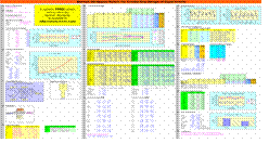
So what method is available to enable engineers conduct more "engineering" design of experiments? The following is a proposed method by the author. First, the full picture may be shown as below or you can download the EXCEL DOE Template L8(2^7) and DOE Template L9(3^4) here.
|
Step1. Name of Researcher
|
|
Many company oriented design of experiments have a team leader and several team members working in the experiments. Here is a logical step to identify the team.
|
|
Ahmad Badrul
|
Step 2. Objective
|
|
What is the purpose of the experiment? This should be clear statement of what needs to be done. Often, clear objectives can be stated, for example: To increase the current flight time of 2.2 seconds to 3.5 seconds for a throw height of 3 metres.
|
|
To achieve high spinning time
|
Step 3. Problem Statement
|
|
What is the problem? Why is this experiment necessary? What is the “burning need?” A problem statement should at least describe the problem faced. Often this can be in the form of engineering short-coming or even a process deficiency, e.g. the post mold cure takes 4 hours because the convention current cannot be achieved earlier.
|
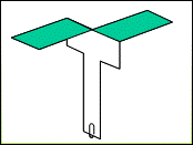
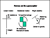
The helicopter spins too fast.
|
Step 4. Quality Characteristics
|
What is to be measured? This is effectively the response. What is this and how is it to be measured? An important aspect of the quality characteristic is whether the response type is smaller-the-better, larger-the-better, nominal-the-best or signed target. The type of characteristic determines the objective target intended. Much of the data analysis later in a design of experiments is determined by the type of quality characteristic.
 |
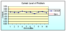
Step 5. Current Level of Problem
|
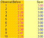
The current level of problem is an indication of the status quo. This should clearly show the current performance of the response being measured. In particular, the target, process mean and variation should be evident from a suitable graphical representation.
|
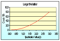
Step 6. Quality Loss Function
|
The quality loss function is often attributed to Taguchi although there is evidence that it may be used earlier without attribution. The quadratic loss function is an approach to quantifying the “average quality loss” based on its deviation from the target. This is often done on a “loss per piece” basis. Many statistics are not at ease with this method. If this is the case, the stakeholder should identify a suitable method of quantifying the loss. After all, the practical need for this loss function quantification is for a comparison of cost savings. Any other reasonable method may be used.
|
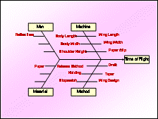
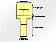
Step 7. Cause-Effect Diagram
|
The cause-effect diagram step allows the team to brainstorm for factors affecting the response. It is not unusual that an optimization be done by an individual. Even in that case, the cause-effect diagram forces the engineer to look for all likely causes that affect the response.
|
Step 8. Parameter-Diagram
|
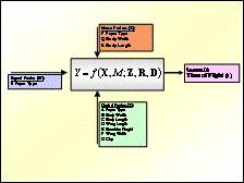
Having identified the likely causes, the next step is to build a Parameter Diagram. This diagram is essentially a short list of factors that can be classified according to its role in the experiment.
|
Step 9. Factors for Study
|
|
Control factors are set by the engineer during the experiment and at the end of the experiment, an optimum condition is sought. Noise factors cannot in fact be set by the engineer, However, noise factors are set during the experiment purely to introduce variability in the experiment and an optimum condition is NOT sought for these factors. Signal factors change the overall effect of the response. They are often included for study in an experiment and no optimum condition is selectable. Instead, the signal value is set according to the user’s condition.
|
In this step therefore, the factor level settings (current and proposed levels) are specified for subsequent experimentation. By factor levels it is meant whether a factor is studied at 2-levels, 3-levels, etc. Although more levels may appear better, since experimental trials increase by a power function, often 2-level factors are suitable for screening experiments and for most practical reasons 3-level factors are sufficient to detect curvature.
 
|
Step 10. Experimental Design
|
|
The Experimental Design step is where the experimental recipes are created. This forms the “table of factor settings” that allow the engineer to construct the experimental trials. In most cases, a good design should include a direct product design consisting of a control factor array and a noise factor array.Data collection then follows the factor settings. Data for experimental trials can be logically and easily entered into a two way array.
|
Many industry standard software jump-start from here with a flash of the selected array and most often with the principal factors. The user will have to learn to use spreadsheet style columns and assign other columns of data to blocks, replicates or noise factor setting apart from having to learn to use factorial points, axial points and center points. Most sanguine users surrender at this point. Yes, sanguine users includes Green and Many Black Belts.


|
Step 11. Response Table
|
Once data is entered, a response table of values indicating the mean effects of the performance indicators, such as the Target Performance Measure (TPM) and Noise Performance Measures (NPM), are calculated. Response tables show some information regarding factor importance, however, they do not show the factor effects relative to the experimental error.

|
Step 12. Analysis of Variance
|
|
|
Step 13. Factor Level Averages
|
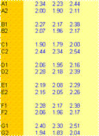
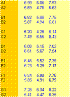
Information from Steps 11 and 12 are combined to generate these tables which show the mean factor levels for the performance measures.
|
Step 14. Response Graphs
|
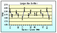
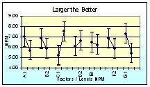
Data from the response tables are not very easily appreciated unless shown as a graphical display. The response graphs display factor effects very clearly. Most engineers will now begin to “feel” the processes they studied.
|
Step 15. Optimum Factor Selection
|
|
Once the analysis of variance is completed and unimportant factors pooled to error, the remaining factors can be considered important towards the response that is being studied.
|
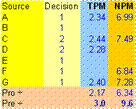
Given the response type in Step 4, optimum conditions can be routinely calculated. Likewise, since the current condition is known from Step 9 it is also possible to include comparisons of the current condition. With a dynamic model, the engineer can evaluate other optimum conditions as required and immediately compare its performance with the recommended optimum condition.Most commercial Design of Experiments software does not come anywhere close to this.

|
Step 16. Predicted Values
|
Even if an engineer conducted full factorial experiments, it is necessary to calculate the response performance at the predicted value (PV), i.e. the optimum condition.

|
Step 17. Confirmation Experiment
|
|
Following the estimation of the predicted value a confirmation experiment (CE) must be conducted with factor level settings as in the optimum condition.In any fractional experiment, there will be many interactions that are not included in the experimental model. If all important factor effects (including any interactions) account for a large contribution (i.e. small experimental error) then CE must be approximately equal to PV. That is:
|
If (all other effects) ≠ 0, then the model has not adequately captured (important factors) and the experiment is said to be not successful. So..? Back to the drawing board.

|
Step 18. Full Scale Implementation
|
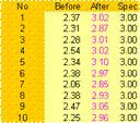
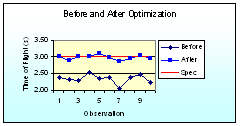
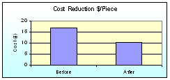
If the Confirmation Experiments verifies the Predicted Value then a control implementation can be done under operating conditions. A series of observations can then be done at the optimum condition. A comparison of “Before” and “After” graphs is drawn to provide a visual impression of the optimization.
|
Step 19. Gain Calculation
|
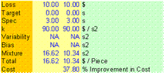
A quantitative gain calculation also needs to be performed so that there is a one-to-one objective or manager’s bottom-line comparison in monetary units. Even a 50% improvement may fail to improve a senior manager if the value of this improvement is only, say 10$ per unit, compared to another improvement of only 10% but with a cost gain of 100$ per unit. Thus, the manager has every need to know both the percentage gain as well as the monetary gain. Monetary gain is best displayed in a bar chart on a 10 – 100% bar height.
|
Step 20. Conclusion.
|
|
Finally, the conclusion. Here, the engineer can summarize any implementation action, lessons learnt and cost savings achieved.And now the ultimate question. Which commercial software does all this and gives you a printed report?
|
If you answered “None” please refer to http://www.ict-m.com.
|
|
Conclusion |
|
Conducting a Design of Experiment does not have to mean sending engineers back to college education. It is possible to have auto-cruise in cars –so - what about auto-cruise in Design of Experiments? Software can be made more intelligent to process the situation required by the engineer rather than to expect the engineer to understand and sometimes discern complex mathematical and statistical abstractions.
|
References
|
|
Belavendram, N. (1995) Quality by Design - Taguchi Techniques for Industrial Experimentation. Prentice Hall, May 1995. ISBN: 0-13-186362-2.
|
Dr
*About the author.
Dr. Nicolo Belavendram is a lecturer with the University of Malaya. He specializes in Robust Design and Technology Development for manufacturing industries.
Dr. Nicolo Belavendram is the author of Quality by Design: Taguchi Techniques for Industrial Experimentation published by Prentice Hall May 1995. He is the Domain Knowledge Expert Consultant in iCT-M software. Please visit the web site at http://www.ict-m.com for more information on Six Sigma / APQP / TQM and the work of the author. You may Email him at info@ict-m.com. Academics and consultants may use iCT-M software for academic and training purposes with his permission.
This article should not be reproduced in any format without prior permission from the author. It is available for academic reprinting with due recognition and reference to the author Dr. Nicolo Belavendram (info@ict-m.com) and iCT-M (http://www.ict-m.com) in its full attribution.
* Do not remove or delete this from this article.
|
|
|
|
|


