Principles of Robust Manufacturing
Principles of Robust Manufacturing
By Dr. Nicolo Belavendram
Faculty of Engineering, University of Malaya
Abstract
Although researchers (scientists, engineers, etc.) may have great skills in their areas of expertise, many however do not possess the skills for conducting systematic research. Often, researchers conduct experiments only on the Target-Performance Measure (e.g. mean) without a consideration of the Noise-Performance Measure (e.g. signal-to-noise ratio). Most experiments are also conducted without suitable cost analysis of the functional performance. Robust Design is a technological breakthrough that enables efficient experimental and simulation methods to optimize product and process design for manufacturability, quality and reliability. The role of Robust Design is to minimize the sensitivity of products and processes to uncontrollable noise factors (e.g. environmental, deterioration and manufacturing). Robust Design achieves this by selecting an objective function and evaluating it to maximize the function with regards to controllable design factors. The evaluation procedure itself uses orthogonal arrays as an efficient analytical method resorting to the 2-step optimization of 1) reducing the variability and 2) adjusting to target. Since engineering optimization come in a variety of problems, several generic design optimizations that can be conducted through Robust Design are explained in this paper.
Keywords
Robust Design, Design of Experiments, Orthogonal arrays, Dynamic Characteristics, Taguchi Methods, Target Performance Measure, Noise Performance Measure, Product Optimization, Process Optimization.
1 Introduction
|
|
|
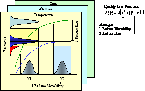
Figure 1.: Principle of Robustization.
|
Robust Design can be said to have its roots in the work done be Sir Ronald Fisher[1] at the Rothamsted Experimental Station where he developed the analysis of variance leading to the science of experimental design. More recently, the methods were expounded by Montgomery[2] in several of his books. In the 1980s, experimental design methods were given a total facelift by Genichi Taguchi[3] with his emphasis on the inclusion of noise factors and popularizing the Robust Design methodology as advocated in this paper. Phadke[4] is a leader in the application of Taguchi methods. Taguchi’s approach has often been criticized as a “cookbook” method particularly with respect to his signal-to-noise ratios. However, a treatment on performance measures independent of adjustment (PerMIA) by Logothetis[5] has given much scope to complement Taguchi’s work. In particular, Taguchi’s contribution of a highly structured approach to experimental design highly suited to engineers in industrial environments is notable and praiseworthy.
2 Engineering Quality
One approach to reduce a product’s or process’s functional variation is to reduce the variability due to the noise factors or eliminate them entirely. Undoubtedly, this is not always feasible or even possible. Indeed, any attempt to reduce the variability caused by noise factors would mean the reduction of the useful range, demanding a tighter manufacturing tolerance or specifying low drift parameters. All these methods quickly raise the cost of the product or process and are inherently not efficient. A better method is to center the design parameters to minimize sensitivity to noise factors through the principle of robustization as shown Figure 1.
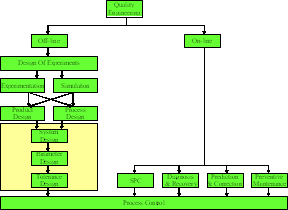
Figure 2.: The Design Process.
Note that during the product design stages, a researcher can robustize a product against all three types of noise factors. During manufacturing process design and actual manufacturing the researcher can only reduce manufacturing imperfections. Once a product is sold, only warranty services can address quality problems. Thus, the quality of a product lies mostly with the product and process design as shown in Figure 2 with an emphasis on three major steps in designing a product or process.
- System design
- Parameter design
- Tolerance design
System design is the workable product or process. Parameter design is the utilization of control factors to minimize sensitivity to noise. Here, wide tolerances are allowed so that costs are a minimum. If Parameter design fails to achieve adequate functional performance, then Tolerance design is used to select factors that minimize variance based on cost effectiveness.
3 Optimization Strategy – Static Characteristics
Product and process optimization have been written and taught in many ways. The author however thinks that the following step-by-step method (see Figure 3) is the best approach for learning product and process optimization particularly for engineers and research students.
3.1 The quality loss function
The current status of a characteristic is often the cause for concern for optimization. For instance, the current performance level of a response is not meeting the target value. A target can be zero (smaller-the-better characteristic), a specified value (nominal-the-best) or infinity (larger-the-better).
The quality of a product can be expressed as the total loss-to-society from the time the product is sold to the customer. This loss is incurred largely due to the deviation of the functional characteristic from the target value and is estimated through the quadratic loss function.
The quadratic loss function can be used to approximate the quality loss in many situations. The quality loss function has been debated in literature but this paper will not discuss this contention. Let us suggest that the quality loss is proportional to the square of the deviation. That is:
 and therefore, and therefore,
 where k is a constant referred to as the quality loss coefficient. It is important to calculate the constant k so that the equation can best approximate the actual loss within the region of interest. This can be a rather difficult though important task. where k is a constant referred to as the quality loss coefficient. It is important to calculate the constant k so that the equation can best approximate the actual loss within the region of interest. This can be a rather difficult though important task.
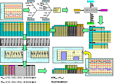
Figure 3.: Step-by-step Robust Design
A convenient way to determine k is to determine first the functional limits for the value of y. A functional limit is the value of y at which half the products would fail in use. Suppose,
 is the functional limits and the loss at this limit is is the functional limits and the loss at this limit is
 . At the specification limit, the loss . At the specification limit, the loss
 and the deviation and the deviation
 then, then,
 . If y is the quality characteristic of a product and t is the target value, then the deviation is . If y is the quality characteristic of a product and t is the target value, then the deviation is
 , and , and
 . .
Notice that when y = t, the loss is zero (or minimum). This is admissible since m is the best value for y. The loss
 increases slowly when we are near t; but rapidly as we go farther away (on either side) from t. This is coherent with the type of behavior we expect the quality loss function to have. The quadratic loss function given above is the simplest mathematical function that has the desired qualitative behavior. increases slowly when we are near t; but rapidly as we go farther away (on either side) from t. This is coherent with the type of behavior we expect the quality loss function to have. The quadratic loss function given above is the simplest mathematical function that has the desired qualitative behavior.
For many pieces, the average loss is
 , where , where

where
 is the sample variance and is the sample variance and
 is the bias squared. We now summarize the loss for a single piece or a sample as shown below. The formula above can be adapted to the smaller-the-better and larger-the-better characteristics as shown in Figure 4. is the bias squared. We now summarize the loss for a single piece or a sample as shown below. The formula above can be adapted to the smaller-the-better and larger-the-better characteristics as shown in Figure 4.
|
Nominal-the-best
|
|

|
|
Smaller-the-better
|
|

|
|
Larger-the-better
|
|

|
|
Figure 4. : Signal-to-noise ratios.
|
3.2 The Cause-Effect diagram
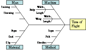
Once the quality loss for the current response is quantified the next step is to identify all the factors that contribute to the deviation of the response from the intended target value. This is done through a brainstorming session together with a Cause-Effect analysis. All aspects of Man, Machine, Method and Material that can possibly affect the Effect recorded.
|
|
|
Figure 5. : Cause Effect diagram.
|
3.3 The P-Diagram
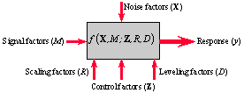
Factors identified in the Cause-Effect diagram can be arranged into three main types of factors namely, Signal factors, Control factors and Noise factors. Other factors such as the Scaling and Leveling factors are special cases of Control factors and are discussed here for completeness.
|
|
|
Figure 6.: The P-diagram.
|
Signal factors (M) are set by the user to attain the desired output. The speed setting in an electric fan, the accelerator of a car, the 0 and 1 in communication systems are all signal factors. Although a researcher can study one or two signal factors in optimization trials, the user will set the factor level according to his/her preference.
Control factors (Z) are the parameter values
set by the researcher. Each control factor is studied at least at two-levels and the parameter design objective is to select the best level. Since there are many control factors in an experiment, the factors are represented in a matrix notation.
Noise factors (X) are not controllable by the researcher or the user. However, for the purpose of optimization, these factors may be set at one or more levels. Since there many be many noise factors in an experiment, these factors are represented in a matrix notation. Obviously, no optimum noise factor is selected in an experiment.
Scaling factors (R) are special cases of control factors that are adjusted to achieve the desired functional relationship as a ratio between the signal factor and the response.
Scaling factors (D) are special cases of control factors that are adjusted to achieve the desired functional relationship as a constant between the signal factor and the response.
3.4 Selection of factor levels
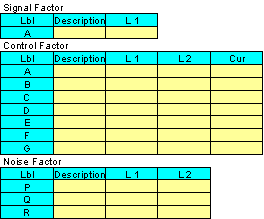
Having decided on the Signal, Control and Noise factors, the factor levels must be identified. In a simple discussion as in this paper, the signal level is set at only one level. The control and noise factor settings are shown Figure 7. A 2-level factor has 1 degree of freedom. If seven 2-level factors need to be studied, then the experimental design must allow at least 7 degrees of freedom. In general an n-level factor has (n-1) degrees of freedom.
|
|
|
Figure 7. : Factors and levels setting.
|
3.5 Selection of Orthogonal Arrays
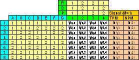
When studying factors, it is important that factors are orthogonal to each other and that they are balanced throughout the study. An orthogonal array[6] is used as the basis for balanced comparisons of several factors. The orthogonal array also simplifies data analysis. Many orthogonal arrays are available with different factor and level combinations. The L8(27) orthogonal array can accommodate seven 2-level factors (i.e. 7 degrees of freedom) in a total of eight experiments. Again, as in factors, an experiment consisting of n trials allows (n-1) degrees of freedom or fair comparisons.
|
|
|
Figure 8.: The L8 orthogonal array.
|
In designing an experiment, it is important to include noise factors to deliberately emulate the effect of noise on the response. This is done by including a noise factor array (preferably also an orthogonal array) across the control factor array. Such a design is called a direct-product design. It is now clear how many data need to be collected, how these will be recorded and analyzed as shown in Figure 8 above.
Experiments are conducted according to the prescription for each trial. For example, in experiment 1, Factors A, B, …, G are all set at level 1. This experimental setting is now exposed to the noise factor combinations in trial 1, i.e. P=1, Q1=1 and R=1, The result under this combination of control and noise factor setting is recorded as y1, 1. The result under y1, 2 is obtained by changing the noise conditions to P=1, Q=2 and R=2 as shown in the array above. Similarly, all the 32 results need to be collected.
3.6 Performance Measures
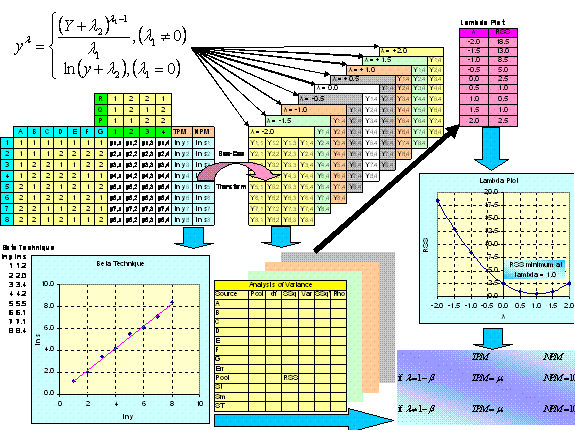
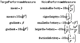
The first part of data analysis involves calculating the Target Performance Measure (TPM) and the Noise Performance Measure (NPM). Common forms of TPM and NPM are defined variously as follows:
|
|
|
Figure 9. : Steps in establishing PerMIA.
|
The choice of which TPM and NPM used depends on the target type of the response characteristic.
The choice of the NPM has been debated in literature. For a more formal statistical approach, the Box-Cox method can be used to identify the best NPM formula to use. This method is based on data transformations using the lambda technique[7]. Although the method is difficult, it can be done on a spreadsheet or suitable software such as iCT-M™.
|
|
|
Figure 10 : Common TPMs and NPMs.
|
3.7 Response Table
To help in subsequent data analysis, the Response Table is completed as follows. To evaluate the effect of factor A on the experiment the averages (or some other measures of location) of A1 and A2 is compared. The average A1 is calculated as,
 for which factor A is in level 1 in the orthogonal array (Experiments 1, 2, 3 and 4. Likewise, average A2 is calculated as, for which factor A is in level 1 in the orthogonal array (Experiments 1, 2, 3 and 4. Likewise, average A2 is calculated as,
 or which factor A is in level 2 (Experiments 5, 6, 7 and 8). The averages for the remaining factors need to be calculated according to the distribution of the levels in the orthogonal array. or which factor A is in level 2 (Experiments 5, 6, 7 and 8). The averages for the remaining factors need to be calculated according to the distribution of the levels in the orthogonal array.
|

|
|
Figure 11.: Response Tables for TPM and NPM.
|
3.8 Analysis of Variance
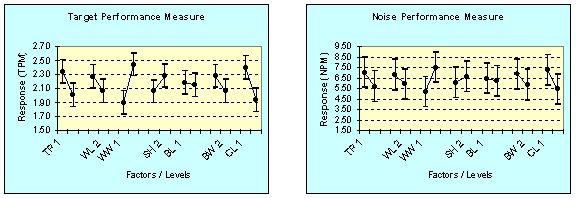
Once the choice of NPM is finalized, the analysis of variance (anova) can be performed easily. For the data above, the number of experiments i=8 and the number of trials j=4. The total sum of squares ST,
|
|
|
Figure 12.: Response graphs of TPM and NPM.
|
 . The sum of squares due to the mean is Sm where . The sum of squares due to the mean is Sm where
 . The corrected sum of squares is St where . The corrected sum of squares is St where
 . The sum of squares due to a 2-level factor is . The sum of squares due to a 2-level factor is
 . The error sum of squares is Se where . The error sum of squares is Se where
 . The variance is calculated as . The variance is calculated as
 and the F-ratio is calculated as and the F-ratio is calculated as
 . Alternatively, the more stable quantity rho is calculated as follows: . Alternatively, the more stable quantity rho is calculated as follows:
 where where
 . .
3.9 Response Graph
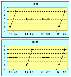
The next step is to visualize the effect of all factors on a common scale against the overall experimental average. The graph below shows clearly the effects of each factor. A factor which has a high gradient (i.e. big difference between level 1 and level 2) is a significant factor. A factor which has a low gradient (i.e. small difference between level 1 and level 2) is an insignificant factor.
From a comparison of the TPM and NPM factor effects, four combinations of factors emerge. These are shown diagrammatically in . Note that this represents the ideal form where factor A largely affects the mean (significant in TPM and insignificant in NPM), factor B largely affects the variance (insignificant in TPM and significant in NPM), factor C affects neither (insignificant in TPM and insignificant in NPM) and factor B affects both (significant in TPM and significant in NPM).

|
|
Figure 13. : Analysis of variances (ANOVA).
|
3.10 Selection Table
|
|
|
Figure 14. :
|
In reality, the optimum factor level selection must be based on the contribution of the factor to the total variance. A condition of selection is that both levels of a factor cannot be chosen at the same time, e.g. A1 to optimize TPM and A2 to optimize NPM as both factors cannot be set simultaneously. Often, since there may be several factors, a Selection Table[8] makes it easier to choose factors. To do this, the TPM factor rank, optimum level and the NPM factor level with its optimum level are tabulated.
The rule is: If the TPM and NPM optimum factor level are the same, select that factor level (since they both optimize the TPM and NPM); otherwise, compare the TPM and NPM ranks and select the optimum factor level based on the higher rank. The Selection Table method may appear redundant when performing smaller-the-better and larger-the-better characteristics. In these cases, the variance is linked to the mean and the use of TPM many not be necessary when variance reduction is emphasized. However, the method above is a more consistent procedure embracing the 2-Step Optimization. A better method would be to include only factors in the included in the analysis of variance above.
The next step is to calculate the Predicted Value for both the TPM and NPM. This is based on the optimum factor levels in the Selection Table.

3.11 Confirmation Experiment
When the optimum factor levels have been selected, the confirmation experiment must be conducted at the selected factor levels. The results of the Confirmation Experiment (CETPM and CENPM) are compared to the Predicted Values (PVTPM and PVNPM respectively). If CETPM = PVTPM then the experiment is said to be additive (significant factors are true) and interactions (all other effects) are negligible. In this case the experimental optimum factor selection can be regarded as reproducible and the optimum factor level settings can be implemented on a larger scale (e.g. production).
|

|
|
Figure 15. : Confirmation experiment.
|
|

|
|
Figure 16. : Selection Table.
|
Sometimes, certain observations during the experiment may lead a researcher to consider a different optimum factor level setting. In this case, the researcher should investigate the combination as another confirmation experiment. In any case, the best of the confirmation experiments should be used as the final optimum condition.
3.12 Before and After Comparison
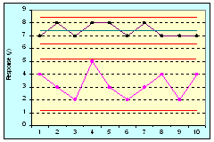
At this stage, the final optimum factor level setting must be implemented on a large scale and the results should be monitored as follows. Here, ten reading at the old factor level setting (Before) is shown against the new factor level setting (After) in Figure 17.
|
|
|
Figure 17. : Before-After Comparison.
|
3.13 Cost savings calculations
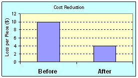
Cost calculations can be conducted to measure the cost savings. Cost calculations show that the quality loss is reduced significantly.
4 Optimization Strategy – Dynamic Characteristics
The Robust Design methodology for static characteristics (signal factor set at one level) can be extended to the dynamic characteristics (signal factor set at two or more levels).
|
|
|
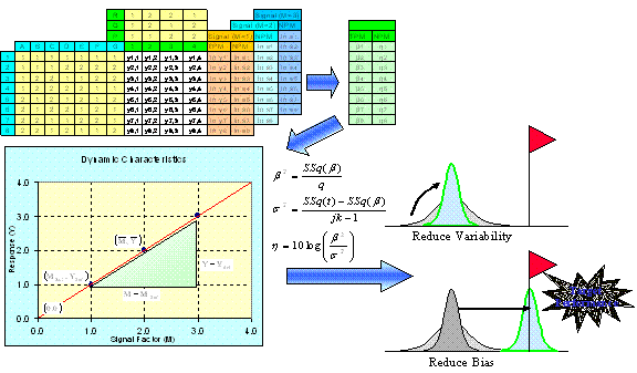
Figure 18.: Schematic of Dynamic Characteristics.
|
Experiments in Dynamic characteristics can be regarded as a series of static characteristic experiments at two or more signal levels. In the static characteristics, the target value is unchanging (i.e. optimization is a point e.g. flight time of 3 sec although this may have a tolerance). In dynamic characteristics the target value is changing (i.e. optimization is a line y = mx + c where for example, y is the time of flight, m is some proportionality constant and x is the distance of throw). Here, the gradient is optimized. Such a method has a vast scope of usage in industrial experimentation.
Dynamic problems are characterized by the presence of signal factors. Depending on the nature of the signal factor and the response variable, there are four common types of dynamic characteristics.
Continuous – Continuous, Continuous – Digital, Digital – Continuous and Digital – Digital.
For the case of Continuous – Continuous, both the signal factor and the response variable are continuous variables. The desired functional relationship is linear and,

Consider the point (M, Y) and a reference point (Mr, Yr). The gradient of this line is
 . Suppose the signal factor M at j levels. Mathematically, . Suppose the signal factor M at j levels. Mathematically,
|
|
|
Figure 19.: Cost reduction.
|
Mj = Number of signal levels (M1, M2, …, Mj). Further, suppose that each experiment is conducted at three noise levels.
Nk = Number of noise levels (N1, N2, N3)
At this point, the passive dynamic characteristic itself may be regarded as three distinct types:
· Case 1:
Reference point (Mr, Yr) = (Mr, Yr), i.e. line passes through reference point.
· Case 2:
Reference point (Mr, Yr) = (0, 0), i.e. line passes through origin.
· Case 3:
Reference point (Mr, Yr) = (Mbar, Ybar), line passes through data mean.
This is the most general case. With the selection of (Mr, Yr) as the reference point, the origin is shifted to (Mr, Yr). Therefore;
True value input = Mr output = Yr
True value input = M - Mr output = Y - Yr
If (Mr, Yr) is the coordinate through which the line passes, the number of units q of m is: therefore, therefore,

Using least squares estimation, the regression sum of squares due to β:
 and and
 while while
 . Thus, . Thus,
 is easily calculated. The general method of analysis for TPM and NPM described earlier can now be used readily. is easily calculated. The general method of analysis for TPM and NPM described earlier can now be used readily.
5 Reference
[1] Fisher, R. A., The Design of Experiments, 7th edition, Oliver and Boyd, 1960.
[2] Montgomery, D. C., Design and Analysis of Experiments, John Wiley and Sons, 1976.
[3] Taguchi, G., System of Experimental Design, Unipub Kraus International Publications, New York, 1987, Volumes 1 and 2.
[4] Phadke, M. S. and Dehnad, K., Optimization of Product and Process Design for Quality and Cost. Quality Reliability Engineering International, April–June 1988, vol. 4, no. 2, pp. 105–12.
[5] Logothetis, Box-Cox Transformations and the Taguchi Method, Appl. Statist. (1990), 39, No. 1, pp. 31-48.
[6] Taguchi, G. and Konishi, S., Orthogonal Arrays and Linear Graphs – Tools for Quality Engineering, ASI Press, 1987.
[7] Logothetis, N., The Role of Data Transformations in Taguchi Analysis. Quality Reliability Engineering International, January–March 1988, vol. 4, no. 1, pp. 49–61.
[8] Belavendram, N, Quality by Design: Taguchi Techniques for Industrial Experimentation, Prentice Hall, May 1995. ISBN: 0-13-186362-2.
Dr
*About the author.
Dr. Nicolo Belavendram is a lecturer with the University of Malaya. He specializes in Robust Design and Technology Development for manufacturing industries.
Dr. Nicolo Belavendram is the author of Quality by Design: Taguchi Techniques for Industrial Experimentation published by Prentice Hall May 1995. He is the Domain Knowledge Expert Consultant in iCT-M software. Please visit the web site at http://www.ict-m.com for more information on Six Sigma / APQP / TQM and the work of the author. You may Email him at info@ict-m.com. Academics and consultants may use iCT-M software for academic and training purposes with his permission.
This article should not be reproduced in any format without prior permission from the author. It is available for academic reprinting with due recognition and reference to the author Dr. Nicolo Belavendram (info@ict-m.com) and iCT-M (http://www.ict-m.com) in its full attribution.
* Do not remove or delete this from this article.
| 


