By Dr. Nicolo Belavendram
Introduction
In any welding procedure, the ideal value of an agreed quality characteristic (or objective characteristic) may be regarded as the target. Typically, there are three types of target: Smaller the better (SB), Nominal the best (NB) and Larger the better (LB). Any deviation from a target causes a loss. Of course, if the system parameters change, the quality characteristic will deviate from the target.
However, deviation from the target can be caused not only by the variations in the system parameters but also noise factors. Noise factors can be variations due to attrition, environmental effects or piece to piece (product to product) differences. From a welding point of view, because it is not possible to have perfect quality (i.e. zero deviation from target) there will be some deviation. The objective of employing experimental design concepts is to identify ways to intrinsically minimise this deviation.
Deviation of the objective characteristic from the intended ideal causes a loss. If an engineer attempts to decrease deviation by using components with very tight tolerances for the initial values and high grade components to reduce attrition or ageing, then this will increase the cost of the product; and still almost nothing could be done to reduce the environmental effect. Thus, at the design stage of a new procedure development, it is important that the settings of nominal parameter levels (and not the tolerances of the parameters) are selected very carefully. The goal is to identify parameter levels such that the objective characteristic is insensitive to noise. Such a method allows the least expensive components to be used and hence a procedure that is not only on-target but also robust.
The aims in this paper are twofold: Firstly, an example of a parameter design study is reported. This is based on a relationship arising in welding presented by Raveendra and Parmar (1987). This type of study was proposed by Taguchi (1986) with an example relating to a wheatstone bridge. Secondly, although the study requires extensive simulation support, the approach presented demonstrates how this was accomplished using a simple macro program in Excel. Thus, specialised computing software is not required.
Principle of Robustisation
The principle of robustisation has been pioneered by Taguchi (1987). This objective of robustisation can be achieved by parameter design. In the case where a mathematical equation models the objective characteristic the Parameter Design can be performed by computer simulation. This is particularly true in electronics where well established and reliable relationships between components and electronic characteristics (e.g. voltage, current) are frequently found. A detailed account of such a Computer Simulated Parameter Design is given by Taguchi (1986) and Taguchi and Wu (1985).
The principle of robustization is based on a two-step approach to
1. reduce the variability
2. reduce the bias as shown in Figure 1
Given a nonlinear relationship between factor A and the output response, it is clear that the setting at A1 transmits much variation to the response whereas the setting at A2 allows only a small variation to be transmitted. Note that the change of the levels in factor A is mere one of setting, e.g. temperature at 100° or 120° and does not require any special treatment or cost. Another factor B may be capable of changing the mean value such that the overall response can be increased or decreased by changing from B1 to B2 (or vice versa).
Consequently, it is vital to identify which of factors A, B, C, …, E affect the mean and which of them affect the variability. This incidentally, is a relatively simple task as shown in Figure 2.
If one can identify factors that largely affect the variability only, then that factor can be used to reduce variation. Similarly, if factor can be identified to largely affect the mean then that factor can be used to reduce bias. Factors that affect neither can be used to select the factor on other criteria (e.g. cost, convenience). Factors that affect both can be a nuisance because changing the mean affects the variability and vice versa. The identification of factor effects can be done through any form of experimentation or simulation.
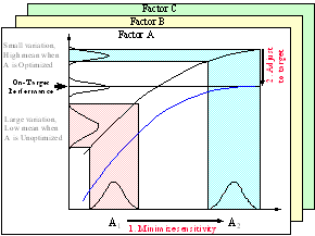
Figure
1. Principle of Robustization.
Figure
2. Factor effects.
In the fabrication and welding industry, the need for increased productivity and improved quality, the shortage of labour and increasingly stringent health and safety requirements have increased the demand for automation to overcome many of the current problems of welded fabrication. Welding robots are one such means, and for arc welding robots, this extends the scope of a semi-automated process to a fully automated one (Raveendra and Parmar, 1987).
To make effective use of arc welding robots it is essential that a high degree of reliability be achieved in predicting the weld bead geometry and shape relations to attain the desired mechanical strength in the weldment. This necessitates that data be represented in the form of an equation or a mathematical model which can be programmed easily and fed to the robot. Raveendra and Parmar (1987) and Gupta and Parmar (1989) have conducted factorial experiments in this area.
In the study by Raveendra and Parmar (1987), the control factors are arc voltage (V), welding current (I), welding speed (S), gun angle (T), and nozzle to plate distance (N). These control factors are used to predict the quality characteristic namely the penetration (P). The equation developed by Raveendra and Parmar (1987) after decoding for levels is:

In the following, a target value for P of 2 mm is taken. For production purposes it is essential not only to predict the quality characteristic P, or by trial and error arrive at acceptable control factor values to achieve a desired P, but to provide a robust set of parameter levels to ensure that the objective characteristic will not vary much even if the system and environmental parameters vary somewhat.
Computer Aided Parameter Design
The problem consists of identifying the factor combination which simultaneously produce a target value of 2 for P and also has a minimum response change in P for small perturbations in the factor values. In this case, even though the non-linearity in P is not marked, achieving this by traditional methods is difficult if not impossible. Two conventional methods that were attempted are the grid-search and the numerical calculus procedure. The former method could identify a factor condition that satisfied the target but there was no consideration for robustness. The latter was mathematically and computationally difficult.
Taguchi (1986) has proposed the parameter design procedure to deal with such a problem. In this case, since a target has been specified for P and variability is to be minimised, the SN (η) ratio is appropriate as a suitable response for analysis where
 is the mean and
 is the standard deviation. Additionally, it is preferable to work with η in the decibel (dB).

Since the SN ratio is proportional to the inverse of the variance of the measurement error, the combination of the parameter levels with the largest SN ratio will have the minimum error variance and this will reflect the optimum design combination. Therefore the SN ratio represents a very powerful statistical tool to determine not only some combination of factor values that gives the required output but also that combination that is least affected by uncontrollable noise factors.

Figure 3. Control and Noise Factor setup.
Figure 4. Direct Product Design.
Experiment and Data Collection
In the simulation experiment that follows, the factors V, I, S, T and N are studied. These factors are assigned various values (levels) as shown in Figure 3.
These factors and levels are assigned to an L36(23x313) orthogonal array readily available from the literature such as Taguchi and Konishi (1987). An orthogonal array is a balanced matrix of factors and levels, such that the effect of any factor or level is unconfounded with any other factor or level. In the L36(23x313) considered, it would be possible to assign 3 two level factors and 13 three level factors in a total of 36 experiments. Another L36(23x313) orthogonal array is built onto the Control Factor Array. This is called the Noise Factor Array and in this case is the transpose of the Control Factor Array. This arrangement shown in Figure 4 is called the direct product design.
During computation, depending on the Control Factor Array level and the Noise Factor Array level, the value assigned to a factor is perturbed by "1% about the mean value. For example, and referring to Figure 3, when the Control Factor Array level is V1 (i.e. mean value of V is 25 volts) the Noise Factor value is ‑1% for level V1,1, "0% for level V1,2 and +1% for level V1,3. Hence, the noise factor value of V at level 1 is 24.75 volts, level 2 is 25.00 volts and level 3 is 25.25 volts. Since all factors are similarly treated, the perturbation in the factor levels is deliberately introduced into the equation for P. Having established all the values Vc,n, Ic,n, Sc,n, Tc,n and Nc,n, where c is the control factor level, and n is the noise factor level, the value of the penetration Pi,j, can be computed where i is the trial number of the Control Factor Array and j is the trial number of the Noise Factor Array.
Example of Computation
From the experimental lay-out, Control Factor Array and Noise Factor Array and Noise Factor set-up around the mean level, the computed matrix P with elements Pi,j give the simulated values for penetration (P-2) with the ith control factor trial and the jth noise factor level trial. For example, the values of V, I, S, T and N for control factor trial row 1 and noise factor trial column 1 (i.e. P1,1) has settings where; V1,1 = 24.75 volts, I1,1 = 247.50 amperes, S1,1 = 247.50 mm/min, T1,1 = 0.0099 degrees and N1,1 = 19.80 mm. Note that i and j refer to the trial number in the direct product design. c and n refer to the factor level settings. The program must then calculate P1,2, P1,3, …, P1,36 so that there are 36 noise factor trial values of P for control factor trial 1. Next, the calculating the following quantities are calculated:

This procedure is then repeated for i = 2 to 36. The Pi• values are then used in the response analysis and anova computations.
This simulation can be programmed in many software macro languages. A spreadsheet such as Excel, can race through these calculations in seconds so that numerical complexity is not an issue at all.
Computations
The mean and SN ratio results were then analysed in terms of the factor effects and the results are shown in Figure 5. This is done by collecting all the P values for a given factor level and calculating the average of that factor level. Subsequently, an Anaylsis of Variance was conducted. This analysis is a standard method discussed in Belavendram (1995). The results of the anova calculations are shown in Figure 6 where Err is the unassigned remaining columns in the control factor array. Df is the degree of freedom of the factor, SSQ is the sum of squares, Var is the variance, SSQ' is the corrected sum of squares and Rho is the percent contribution for the identified factors.
Pooling of non-significant factors is done on all factors with a contribution ratio of less than 5%. Err is not a factor, nevertheless, since the mean response at different ‘factor levels’ for Err is similar; this shows that there is little (13.29 %) residual error effect left to be estimated. The analysis of variance shows that the factors T is the most important (46.1%) followed by V (20.4%) and I (20.1%), i.e. they have large contribution (Rho %) values.
Referring to Figure 5, the factors levels to be selected are V3, I2 and T3. From Figure 3, the choice of optimum levels is therefore V = 35 volts, I = 305 amperes and T = 30 degrees. The remaining factors (S and N) do not greatly influence the SN ratio. Since P depends on V, I, S, T and N, having selected values for V, I and T, the level for the non-significant factors S and N, can be chosen on other constraints (e.g. economic or convenience) to adjust to the required value of P, i.e. nominal value of P.
Figure 5. Graphs of mean and SN ratio.
Figure 7. Results of Parameter Optimization.