|
|
DOE Guidesheet 2
|
DOE Guidesheet 2:
DOE – Improving Product and Process – Advanced
|
|
|
|
What is DOE?
|
|
In manufacturing Industries, experimentation is essential for gaining information about process or a product. The traditional approach of experimentation is the one-variable-at-a-time approach (henceforth referred to as OVAT) in which all of the variables that could possibly affect the quality or the performance of the process or product are held fixed except for one. This variable is changed until its best setting is found. It is then held fixed at this setting. The same thing is then done for a third variable, a fourth variable, etc.
The modern approach of experimentation is known as design of experiments (henceforth referred to as DOE). In DOE, the variables are varied simultaneously in pre-determined combinations. The data obtained from the experiment is analyzed using statistical methods in order to obtain objective conclusions. Such analysis can be easily done using statistical or business softwares that are available commercially. Often, the analysis is done manually using graphs and simple calculations. DOE is also known as statistical design of experiments since it is based on sound statistical practices.
Compared to OVAT, DOE involves a smaller number of runs, thereby reducing the cost and amount of time required for the experiment. The conclusions obtained from DOE is also more accurate since OVAT may cause you to miss the best settings if the variables interact, that is if the effect of a variable on the quality or performance of a process or product depends on the setting of another variable(s). We will elaborate more on this in the section titled 'Detecting interactions using DOE'.
DOE encompasses a wide range of techniques such as factorial designs, fractional factorial designs, response surface methodology, evolutionary operation (EVOP), etc. The choice of which technique to use depends on the objectives of the experiment, the amount of available resources, the nature of the process that is to be experimented on, etc. Factorial designs are straightforward and easy to use, and are good starting point for learning DOE.
Other more advanced designs such as fractional factorial designs and response surface methodology can be easily understood once you have acquired a good understanding of factorial designs. In fact, many people think of DOE as factorial designs.
|
What is DOE used for?
|
|
The earliest documented use of DOE in the manufacturing industries can be traced back to as early as the 1920s, and can be found in the works of L.C.H. Tippet (1943). The latter contained actual examples of the use of DOE in the textile, electrical, mechanical, and foundry industries in Britain . Nowadays, the use of DOE can also be found in a wide range of manufacturing industries such as electronic, food, chemical, paper, automotive, and rubber industries in addition to those mentioned by Tippett.
One of the uses of DOE in the manufacturing industries is for troubleshooting manufacturing problems. An actual example of this can be found in Czirtrom et al. (1998). In the latter, a bottleneck was created in a semiconductor manufacturing plant when one particular furnace could not be used to oxidize silicon wafers due to excessive variability in oxide thickness. There was too much variability from site to site on each wafer to wafer in each furnace run. An experiment was performed using DOE to search for processing conditions that minimized the variability, while taking the mean oxide thickness to its target value of 200 Angstrom.
Three variables; hydrogen flow into the furnace, the ratio of the hydrogen flow to the oxygen flow, and heat plug (on or off) were included in the experiment. For the first two variables, two levels; a low and high level, were investigated. Twelve runs were performed, as shown in Table 1.
|
|
|
|
Run
|
Hydrogen Flow
|
Hydrogen to Oxygen Ratio
|
Heat Plug
|
|
1
2
3
4
5
6
7
8
9
10
11
12
|
M
H
H
L
L
M
H
H
L
L
M
M
|
H
L
H
H
L
M
L
H
H
L
M
H
|
On
On
On
On
On
On
On
Off
Off
Off
Off
On
|
|
L:
|
low level of the respective variable
|
|
H:
|
high level of the respective variable
|
|
M:
|
mid-point of the low and high levels of the respective variable
|
|
|
|
Runs 1 and 12 are at the standard oxidation operating conditions. Runs 2 to 5 were performed in a random order with the heat plug on. Runs 7 to 10 were performed in a random order with heat plug off. We say that runs 2, 3, 4, 5, 7, 8, 9, and 10 constitute a full fractional design with three variables at two levels each. The experiment was performed twice.
For each of the runs, oxide thickness was measured on twelve wafers, and at 13 sites on each wafer. Form a graphical analysis of the data obtained from the runs, the manufacturer was able to determine that the variability could be reduced and the mean oxide thickness could be maintained at the target value with the following processing conditions; high level of hydrogen flow, low level of hydrogen to oxygen ratio, and heat plug on.
Another use of DOE is for determining the critical variables in the process (either an existing one or one that is about to be developed) with the ultimate aim of obtaining the best settings for such variables, that is process characterization followed by process optimization. An actual example of this can be found in Montgomery (1997, 319 : 327). In this example, a chemical product is produced in a pressure vessel. An experiment is carried out in a pilot plant to study the variables thought to influence filtration rate of this chemical product (gal/hr).
The variables are temperature. pressure, concentration of formaldehyde, and stirring rate. Each of them is tasted at two levels; a low level and high level. Sixteen runs were performed, as shown in Table 2 below:
|
|
Table 2: Details of Runs
|
|
Run
|
Temperature
|
Pressure
|
Concentration
|
Stirring Rate
|
|
1
2
3
4
5
6
7
8
9
10
11
12
13
14
15
16
|
L
H
L
H
L
H
L
H
L
H
L
H
L
H
L
H
|
L
L
H
H
L
L
H
H
L
L
H
H
L
L
H
H
|
L
L
L
L
H
H
H
H
L
L
L
L
H
H
H
H
|
L
L
L
L
L
L
L
L
H
H
H
H
H
H
H
H
|
|
L: low level of the respective variable
H: high level of the respective variable
|
|
|
The 16 runs were performed in a random order. We can say that runs 1 to 16 constitute a full fractional design with 4 variables at two levels each. Although it is recommended in DOE that experiments be performed more than once, this experiment was only performed once, presumably because of the high cost of the experiment. The process engineer is interested in maximizing the filtration rate. The engineer would also like to reduce the formaldehyde concentration as much as possible. Both graphical and statistical analyses of the data obtained from the runs indicate temperature, concentration and stirring rate as the critical variables; and that the best filtration rates occur when temperature and stirring rate are at the high level, and concentration is at the low level. Pressure can be at either at the low or high level.
Genichi Taguchi, a Japanese engineer, promoted the use of DOE at the product and process design stages. In so doing, Taguchi made DOE a part of the engineering design toolkit. Taguchi's approach to the use of DOE has been referred to as Taguchi Methods or Robust Designs . For the latter, Taguchi developed tables known as orthogonal arrays for determining the minimum number of runs for the experiment. The tables are based on a particular type of DOE technique known as fractional factorial designs. Taguchi emphasizes the need for investigating the average quality of product as well as the variability in the quality of the products. Taguchi also emphasizes that quality and customer satisfaction can economically be achieved when the average quality of products are as close as possible to their targeted quality levels and the variability of the products around their targeted quality levels are minimal i.e. "On-target and with minimum variance".
The use of Taguchi Methods for designing and producing products that perform well over reasonably wide ranges of application, environment, and utilization methods has become very popular among the engineers in Japan and also in America . An actual application, as related to us by Professor Dennis Kehoe from the University of Liverpool, United Kingdom (Kehoe, 2000), is given in the Appendix (see 'Actual Example of Robust Designs').
However, there are several aspects of Taguchi Methods that have been said to be controversial such as its inability to test for certain important interactions between the variables. We will elaborate more on this in the nest section. Further details of Taguchi Methods can be obtained from Roy (1990), Ross (1988), Taylor (1991), and Montgomery (1997).
|
|
Detecting Interactions Using DOE
|
|
Variables that interact exist all around us. For example, during the dry season, adding fertilizer but no water to flowering plants will kill them. However, adding water and fertilizer will make the plants really bloom. Fertilizer and water interact. The effect of fertilizer on the plants depends on the level of water. At low water level, fertilizer is harmful but at high level, fertilizer is beneficial.
The discoveries of variables that interact have led to breakthroughs in process efficiency and product quality. On the other hand, the lack of discoveries of such variables have been the cause of quality problems. Only by using DOE can we discover such variables. The data obtained from using DOE can be plotted on what is known as an 'interaction plot'. The pattern formed on the plot indicates whether or not interaction exists between the variables. We will illustrate this using actual data, as shown in Table 3
|
|
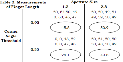
Table 3 : Measurements Of Finger Length
|
|
|
|
Circled numbers indicate average length of the respective corner angle threshold-aperture size combination.
The data was obtained from an experiment that was designed and conducted at Universiti Sains Malaysia on a machine vision system. The DOE technique known as factorial designs was used (Oh, 1995). The system was used to measure the length of the fingers of rubber gloves (in pixel). Here, we are interested in investigating if two of the variables in the system i.e. the aperture chosen for each of the variables, as can be seen in Table 3.
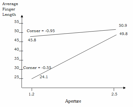
The 32 measurements in Table 3 were obtained in a random manner. The measurements represent the length of the middle finger of a single rubber glove. The actual length was 50 pixels. Figure 1 shows a plot of the average length of each corner angle threshold and aperture size combination (known as interaction plot).
|
|
Figure 1: Interaction Plot of Aperture Size and Corner Angle Threshold
|
|
|
|
Notice that the two lines on the interaction plot are not parallel. This indicates the presence of interaction between aperture size and corner angle threshold. Had the lines been parallel or close to being parallel, we would say that aperture size and corner angle threshold did not interact. Our third guidesheet 'Understanding Factorial Designs' contains more details on how to interpret interaction plots.
Beside interaction plots, more formal statistical techniques can be used to detect interaction such as analysis of variance, p-value and confidence interval analysis. We will illustrate these techniques in our guidesheet titled 'Analyzing Factorial Designs Using More Formal Statistical Methods'. Montgomery (1997) as well as other textbooks on DOE gives details of these techniques.
When using Taguchi Methods, one may need to sacrifice the testing of interactions that may turn out to be important in order to minimize the number of runs for the experiment. While the testing of every possible interactions is usually unnecessary such as the testing of interactions between three (also known as three-term interactions) or more variables, the testing of possible interactions between two variables (also known as two-term interactions) is considered important in DOE. In a three-term interaction, the value of the two-term interaction is dependent on the level of the third variable. Usually, good knowledge of the process is necessary when using Taguchi Methods since one is then able to discriminate between two-term interactions that are not important and those that are.
Two-term interactions have been found to be the cause of quality problems. For example, in the case of Czirtrom et al. (1998) (see page 3 of guidesheet), interaction between hydrogen flow and hydrogen to oxygen ratio was found to be the cause of excessive variability in oxide thickness of the wafers.
|
|
Myths and Realities of DOE
|
|
There are many misconceptions surrounding DOE such as: DOE is not applicable to smaller companies, nor is it applicable to complex processes; DOE is difficult to use; it is exclusively for quality specialists; and it is necessary to stop production when using DOE.
In reality, DOE is applicable to any company; large or small, that needs to improve the quality of its products or to design reliable products in order to compete effectively in both domestic and international markets. DOE can be applied to not only simple processes, but also to complex processes that involve many variables. In an actual case, a manufacturer of wire mesh screens used in the production of microcircuits used DOE (in particular, fractional factorial designs) to investigate the effect of 12 variables on the quality of a new mechanized coating process (Finn, 1987).
Using DOE is like driving a car or using a computer! You can use them and understand the essential principles without knowing the theory behind them. With some training and guidance, you will be able to use DOE easily. With the availability of statistical or business softwares, the analysis of the data can be carried quickly.
A simple DOE technique known as Evolutionary Operation (EVOP) enables you to use DOE without disrupting production. This technique, developed by George Box, has been widely used in the chemical industry in the West (Box & Draper, 1969). Basically, it involves the operator making small changes in the levels of the operating variables until the optimal operating conditions are arrived at. Large changes in the levels of the operating variables are avoided so as to prevent large changes in the performance of the process such as the production of scrap or increased cycle time. Further information about EVOP can be obtained from Box & Draper (1969) and Montgomery (1997).
|
References
|
|
[1] Box, G. E. P & Draper, N. R. (1969) Evolutionary Operation A Statistical Method for Process Improvement , John Wiley & Sons Inc., New York.
|
|
[2] Czitrom, V., Mohammadi, P., Flemming, M., and Dyas, B. (1998) Robust Design Experiment to Reduce Variance Components, Quality Engineering , Vol. 10, issue 4, pp. 645 - 655.
|
|
[3] Finn, L., Kramer, T., and Reynard, S. (1987) Design of Experiments: Shifting Quality Improvements Into High Gear , Joiner Associates Inc., Madison , Wisconsin .
|
|
[4] Kehoe, D.F. (2000) Industrial Applications of Quality Tools, Tutorial Presentation, Regional Symposium on Quality and Automation, 4-5 May, Penang , Malaysia .
|
|
[5] Montgomery, D. C. (1997) Design and Analysis of Experiments , Fourth edition, John Wiley & Sons Inc., Singapore.
|
|
[6] Oh, S. H. (1995) Quality Control and Machine Vision System, Final year Project Report, School of Industrial Technology , Universiti Sains Malaysia .
|
|
[7] Ross, P. J. (1988) Taguchi Techniques for Quality Engineering, McGraw-Hill Book Company, Singapore .
|
|
[8] Roy, R. (1990) A Primer on the Taguchi Method, Van Nostrand Reinhold , New York .
|
|
[9] Taylor , W. A. (1991) Optimization & Variation Reduction in Quality, McGraw-Hill, Inc., New York .
|
|
[10] Tippett, L. C. H. (1943) Statistical Methods in Industry, Iron and Steel Industrial Research Council, British Iron and Steel Federation, Richard Clay and Company Ltd., Bungay, Suffolk, England, as reported by Soren, B. (1992) Industrial Use of Statistically Designed Experiments: Case Study Reference and Some Historical Anecdotes, Quality Engineering, Vol. 4 Issue 4, pp. 547 - 562.
|
|
|
|
|
|